Defining Accurate Floating Coordinate Reference Systems for Legacy Crow Canyon Projects
Kyle Bocinsky
8/20/2020
floating-grid-trigonometry.Rmd
library(localgrid)The Crow Canyon Archaeological Center utilizes local, arbitrary spatial grids for their excavation projects in order to simplify record-keeping and protect the location of cultural sites. These grids are often built off of a primary datum and are intended to be oriented to true north. The primary datum is often (though not always) assigned the false easting and northing of (500,500), and project coordinates are taken in reference to the primary datum. Secondary datums have historically been established as backsights, and grid stakes set using a total station. These local grids are not perfectly aligned to true north, however, and there hasn’t historically been a consistent process for transforming the floating grid coordinates into geographic coordinates or other coordinate reference systems (CRSs).
Here, I describe a method for defining a projected coordinate reference system (CRS) for each CCAC legacy project that will correspond to the project’s floating grid. Associating this CRS to floating grid coordinates will allow for transformation to other CRSs, including UTM, Colorado State Plane, and geographic coordinates.
Target CRS: Oblique Mercator
We define our target CRS as a parameterization of the Oblique Mercator Projection (OMerc), a generalization of the Mercator projection where the ellipsoidal Earth is projected on a cylinder tilted at an arbitrary angle to the equator (i.e., neither along the equator or a meridian). OMerc is useful at local scales, with minimal distortion out to hundreds of kilometers from the point of origin. In the PROJ cartographic projection system, OMerc is defined with the following parameters that we will utilize here:
- lonc (\(lon_0\)): Longitude of the primary datum
- lat_0 (\(lat_0\)): Latitude of the primary datum
- alpha (\(\alpha\)): Azimuth (rotation) of centerline clockwise from north at the center point of the line
- k_0 (\(k_0\)): Scale factor
- x_0 (\(x_0\)): False easting
- y_0 (\(y_0\)): False northing
The values of several of these parameters are trivial — \(lon_0\) and \(lat_0\) are the geographic coordinates of the primary datum (preferably shot using a very high precision GPS receiver), and \(x_0\) and \(y_0\) are the coordinates of the primary datum in the floating grid (often 500,500 in Crow Canyon grids). However, deriving the rotation \(\alpha\) and scale factor \(k_0\) requires a bit of fundamental trigonometry.
Calculating rotation and scaling parameters: The two-point approach
Here, we use high-precision geographic and floating coordinates for the primary datum and a secondary point on our floating grid in order to establish the rotation and scaling parameters for our floating CRS. In summary, the method first projects geographic coordinates into an un-rotated/un-scaled OMerc projection, then calculates the rotation and scaling parameters by applying rotation and scaling transformations to the projected geographic coordinates so that they conform to their floating counterparts.
Selecting points
This method requires high-precision geographic (latitude/longitude) coordinates for two points in the floating grid: the primary datum about which rotation needs to occur, and a secondary point that must be a fixed point of known coordinates in the floating grid. This can be a secondary datum, grid stake, or fresh point shot with a total station using the primary datum and a back-sight. As a rule of thumb, a secondary point that is far from the primary datum (i.e., hundreds of meters away) may provide more precision for calculating the rotation and scaling parameters than a point that is closer to the datum.
pts_geo <-
  sf::st_sfc(
    list(
      sf::st_point(c(-108.510, 37.385)),
      sf::st_point(c(-108.511, 37.384))
    ),
    crs = 4326)

pts_float <-
  sf::st_sfc(
    list(
      sf::st_point(c(500,500)),
      sf::st_point(c(360,380))
    )
  )
For this example we’ll use two points from a fictional site. The differences between the floating and geographic coordinates are greatly exaggerated in this example, and all coordinates are rounded to three decimal places. For a real application, you would want much higher precision geographic coordinates… preferably out to 6 decimal places or more. Coordinates are given in (x,y) format.
- Primary datum: Floating (500,500); Geographic (-108.51,37.385)
- Secondary point: Floating (360,380); Geographic (-108.511,37.384)
Transforming geographic coordinates into an un-rotated/unscaled OMerc projection
Here, we define an un-rotated/un-scaled OMerc projection centered at the primary datum and aligned to true north, and then transform the geographic coordinates for both the primary datum and the secondary point to the units of the OMerc projection. This will allow us to directly compare the un-rotated/un-scaled floating coordinates with the actual floating grid, and calculate the rotation and the scaling factor.
as_proj <- function(x){
  x %>%
    {paste0("+",names(.),"=",., collapse = " ")}
}

datums_omerc <-
  list(proj = "omerc",
       lat_0 = sf::st_coordinates(pts_geo[[1]])[,'Y'],
       lonc = sf::st_coordinates(pts_geo[[1]])[,'X'],
       alpha = 0,
       gamma = 0,
       k_0 = 1,
       x_0 = 500,
       y_0 = 500
  ) %>%
  as_proj() %>%
  sf::st_crs()

pts_geo_float <-
  pts_geo %>%
  sf::st_transform(datums_omerc)
The un-rotated/un-scaled OMerc projection can be defined in the PROJ system as +proj=omerc +lat_0=37.385 +lonc=-108.51 +alpha=0 +gamma=0 +k_0=1 +x_0=500 +y_0=500. Transforming the geographic coordinates for both points to the un-rotated/un-scaled OMerc projection yields coordinates in the same units as the floating grid, with the primary datum at (500,500), and the secondary point at (411.438,389.016) (the coordinates are rounded to the nearest millimeter). Note that the secondary point is at very different coordinates than in the floating grid.
library(ggplot2)
tibble::tibble(
  point = factor(x = c("Primary Datum",
                       "Floating Point",
                       "Geographic Point"),
                 levels = c("Primary Datum",
                            "Floating Point",
                            "Geographic Point"),
                 ordered = TRUE),
  geom = c(pts_float, pts_geo_float[2])
) %>%
  sf::st_as_sf() %>%
  ggplot(aes(color = point,
             shape = point,
             size = point)
  ) +
  geom_sf() +
  theme_minimal() +
  scale_color_manual(values = c("black","black","red")) +
  scale_shape_manual(values = c(17, 19, 19)) +
  scale_size_manual(values = c(3, 2, 2)) +
  theme(legend.title = element_blank(),
        legend.position = "bottom",
        axis.title = element_blank())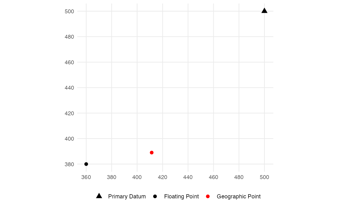
Calculating the rotation parameter \(\alpha\)
The rotation parameter \(\alpha\) is defined as the angular difference from the primary datum to each of the secondary points, in degrees. We can use basic trigonometry to calculate the angle of each point from the \(x\) axis, \(\theta\), of the secondary points, such that \(\theta = {\rm atan2}(y_0-y_1,x_0-x_1)\), where \((x_0,y_0)\) is the coordinate of the primary datum in the floating grid [here (500,500)], and \((x_1,y_1)\) is the coordinate of the secondary point. We subtract the \(\theta_g\) for the geographic coordinates from \(\theta_f\) for the floating coordinates, and then multiply by \(\frac{180}{\pi}\) to convert from radians to degrees.
\[\begin{align} \theta_g &= {\rm atan2}(y_{0}-y_{g1}, x_{0}-x_{g1}) \\ \theta_g &= {\rm atan2}(500 - 389.016, 500 - 411.438) \\ \theta_g &= {\rm atan2}(110.984, 88.562) \\ \theta_g &= 0.897 \\ \\ \theta_f &= {\rm atan2}(y_{0}-y_{f1}, x_{0}-x_{f1}) \\ \theta_f &= {\rm atan2}(500 - 380, 500 - 360) \\ \theta_f &= {\rm atan2}(120, 140) \\ \theta_f &= 0.709 \\ \\ \alpha &= \theta_f - \theta_g \\ \alpha &= -0.189 \times \frac{180}{\pi} \\ \alpha &= -10.81 \end{align}\]
theta_g = atan2(500 - sf::st_coordinates(pts_geo_float[[2]])[,'Y'],
                500 - sf::st_coordinates(pts_geo_float[[2]])[,'X'])

theta_f = atan2(500 - sf::st_coordinates(pts_float[[2]])[,'Y'],
                500 - sf::st_coordinates(pts_float[[2]])[,'X'])

alpha =
  (atan2(500 - sf::st_coordinates(pts_float[[2]])[,'Y'],
         500 - sf::st_coordinates(pts_float[[2]])[,'X']) -
     atan2(500 - sf::st_coordinates(pts_geo_float[[2]])[,'Y'],
           500 - sf::st_coordinates(pts_geo_float[[2]])[,'X']))

alpha_deg <- (180/pi) * alpha
library(ggforce)
tibble::tibble(
  point = factor(x = c("Primary Datum",
                       "Floating Point",
                       "Geographic Point"),
                 levels = c("Primary Datum",
                            "Floating Point",
                            "Geographic Point"),
                 ordered = TRUE),
  geom = c(pts_float, pts_geo_float[2])
) %>%
  sf::st_as_sf() %>%
  ggplot(aes(color = point,
             shape = point,
             size = point)
  ) +
  geom_arc(aes(x0 = 500,
               y0 = 500,
               r = 20,
               start = pi,
               end = (3*pi/2) - theta_g),
           size = 0.5,
           color = "red",
           lineend = "butt") +
  geom_text(aes(x = 500 + 20*cos((3*pi/2) - theta_g/2),
                y = 500 + 20*sin((3*pi/2) - theta_g/2)),
            label = expression(theta["g"]),
            hjust = -0.15,
            vjust = -0.15,
            color = "red",
            size = 5) +
  geom_arc(aes(x0 = 500,
               y0 = 500,
               r = 25,
               start = pi,
               end = (3*pi/2) - theta_f),
           size = 0.5,
           color = "black",
           lineend = "butt") +
  geom_text(aes(x = 500 + 25*cos((3*pi/2) - theta_f/2),
                y = 500 + 25*sin((3*pi/2) - theta_f/2)),
            label = expression(theta["f"]),
            hjust = 1.15,
            vjust = 1.15,
            color = "black",
            size = 5) +
  geom_arc(aes(x0 = 500,
               y0 = 500,
               r = 30,
               start = (3*pi/2) - theta_g,
               end = (3*pi/2) - theta_f),
           size = 0.5,
           color = "dodgerblue",
           lineend = "butt") +
  geom_text(aes(x = 500 + 30*cos((3*pi/2) - mean(c(theta_g,theta_f))),
                y = 500 + 30*sin((3*pi/2) - mean(c(theta_g,theta_f)))),
            label = expression(alpha),
            hjust = 0.5 + 0.65*cos(mean(c(theta_g,theta_f))),
            vjust = 0.5 + 0.65*sin(mean(c(theta_g,theta_f))),
            color = "dodgerblue",
            size = 5) +
  geom_segment(aes(x = 500,
                   y = 500,
                   xend = sf::st_coordinates(pts_float[[2]])[,'X'],
                   yend = sf::st_coordinates(pts_float[[2]])[,'Y']),
               size = 0.5,
               color = "gray70") +
  geom_segment(aes(x = 500,
                   y = 500,
                   xend = sf::st_coordinates(pts_geo_float[[2]])[,'X'],
                   yend = sf::st_coordinates(pts_geo_float[[2]])[,'Y']),
               size = 0.5,
               color = "gray70") +
  geom_sf() +
  theme_minimal() +
  scale_color_manual(values = c("black", "black", "red")) +
  scale_shape_manual(values = c(17, 19, 19)) +
  scale_size_manual(values = c(3, 2, 2)) +
  theme(legend.title = element_blank(),
        legend.position = "bottom",
        axis.title = element_blank())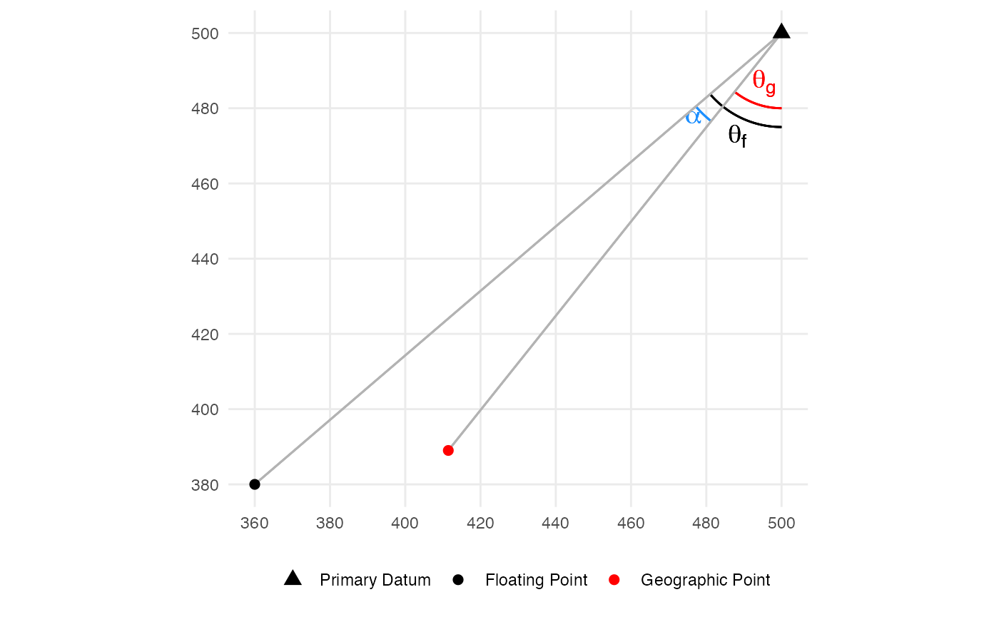
After rotation, the geographic secondary point aligns to the same ray from the primary datum as the floating secondary point.
rotated_omerc <-
  list(proj = "omerc",
       lat_0 = sf::st_coordinates(pts_geo[[1]])[,'Y'],
       lonc = sf::st_coordinates(pts_geo[[1]])[,'X'],
       alpha = alpha_deg,
       gamma = 0,
       k_0 = 1,
       x_0 = 500,
       y_0 = 500
  ) %>%
  as_proj() %>%
  sf::st_crs()

pts_geo_rotated <-
  pts_geo %>%
  sf::st_transform(rotated_omerc)

tibble::tibble(
  point = factor(x = c("Primary Datum",
                       "Floating Point",
                       "Geographic Point"),
                 levels = c("Primary Datum",
                            "Floating Point",
                            "Geographic Point"),
                 ordered = TRUE),
  geom = c(pts_float,
           pts_geo_rotated[2])
) %>%
  sf::st_as_sf() %>%
  ggplot(aes(color = point,
             shape = point,
             size = point)
  ) +
  geom_segment(aes(x = 500,
                   y = 500,
                   xend = sf::st_coordinates(pts_float[[2]])[,'X'],
                   yend = sf::st_coordinates(pts_float[[2]])[,'Y']),
               size = 0.5,
               color = "gray70") +
  geom_segment(aes(x = 500,
                   y = 500,
                   xend = sf::st_coordinates(pts_geo_rotated[[2]])[,'X'],
                   yend = sf::st_coordinates(pts_geo_rotated[[2]])[,'Y']),
               size = 0.5,
               color = "gray70") +
  geom_sf() +
  theme_minimal() +
  scale_color_manual(values = c("black", "black", "red")) +
  scale_shape_manual(values = c(17, 19, 19)) +
  scale_size_manual(values = c(3, 2, 2)) +
  theme(legend.title = element_blank(),
        legend.position = "bottom",
        axis.title = element_blank())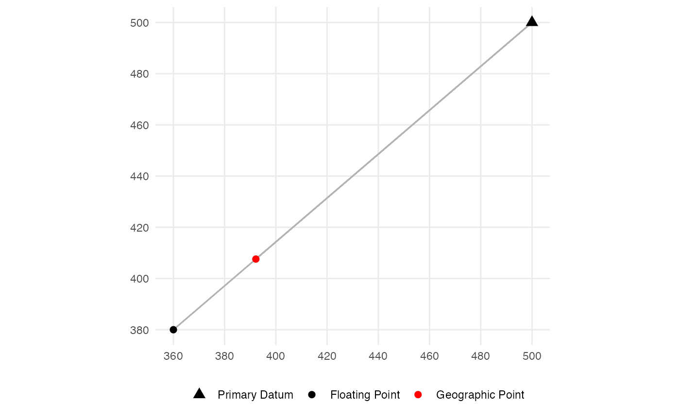
Calculating the scaling parameter \(k_0\)
The scaling parameter \(k_0\) is defined as the scaler required for the distance \(d_g\) from the secondary point in geographic coordinates to the primary datum to equal the distance \(d_f\) from the secondary point in floating coordinates to the primary datum. We use the standard Cartesian distance calculation, \(d = \sqrt{(y_1 - y_0)^2 + (x_1 - x_0)^2}\).
\[\begin{align} k_0 \times d_g &= d_f \\ k_0 &= \frac{d_f}{d_g} \\ k_0 &= \frac{\sqrt{(380 - 500)^2 + (360 - 500)^2}}{\sqrt{(389.016 - 500)^2 + (411.438 - 500)^2}} \\ k_0 &= \frac{184.391}{141.989} \\ k_0 &= 1.299 \end{align}\]
k_0 = sqrt((sf::st_coordinates(pts_float[[2]])[,'Y'] - sf::st_coordinates(pts_float[[1]])[,'Y'])^2 + (sf::st_coordinates(pts_float[[2]])[,'X'] - sf::st_coordinates(pts_float[[1]])[,'X'])^2) / sqrt((sf::st_coordinates(pts_geo_float[[2]])[,'Y'] - sf::st_coordinates(pts_geo_float[[1]])[,'Y'])^2 + (sf::st_coordinates(pts_geo_float[[2]])[,'X'] - sf::st_coordinates(pts_geo_float[[1]])[,'X'])^2)
tibble::tibble(
  point = factor(x = c("Primary Datum",
                       "Floating Point",
                       "Geographic Point"),
                 levels = c("Primary Datum",
                            "Floating Point",
                            "Geographic Point"),
                 ordered = TRUE),
  geom = c(pts_float,
           pts_geo_float[2])
) %>%
  sf::st_as_sf() %>%
  ggplot(aes(color = point,
             shape = point,
             size = point)
  ) +
  geom_segment(aes(x = 500,
                   y = 500,
                   xend = sf::st_coordinates(pts_float[[2]])[,'X'],
                   yend = sf::st_coordinates(pts_float[[2]])[,'Y']),
               size = 0.5,
               color = "black") +
  geom_text(
    aes(
      x = mean(c(500,sf::st_coordinates(pts_float[[2]])[,'X'])),
      y = mean(c(500,sf::st_coordinates(pts_float[[2]])[,'Y']))
    ),
    label = expression(d[f]),
    hjust = 1.15,
    vjust = -0.15,
    color = "black",
    size = 5) +
  geom_segment(aes(x = 500,
                   y = 500,
                   xend = sf::st_coordinates(pts_geo_float[[2]])[,'X'],
                   yend = sf::st_coordinates(pts_geo_float[[2]])[,'Y']),
               size = 0.5,
               color = "red") +
  geom_text(
    aes(
      x = mean(c(500,sf::st_coordinates(pts_geo_float[[2]])[,'X'])),
      y = mean(c(500,sf::st_coordinates(pts_geo_float[[2]])[,'Y']))
    ),
    label = expression(d[g]),
    hjust = 1.15,
    vjust = -0.15,
    color = "red",
    size = 5) +
  geom_sf() +
  theme_minimal() +
  scale_color_manual(values = c("black", "black", "red")) +
  scale_shape_manual(values = c(17, 19, 19)) +
  scale_size_manual(values = c(3, 2, 2)) +
  theme(legend.title = element_blank(),
        legend.position = "bottom",
        axis.title = element_blank())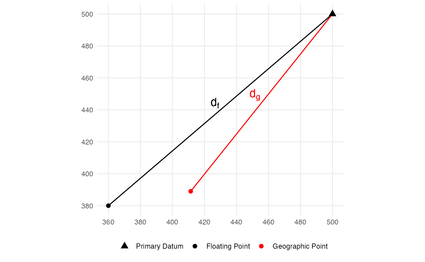
After scaling, the geographic secondary point is the same distance from the primary datum as the floating secondary point.
scaled_omerc <-
  list(proj = "omerc",
       lat_0 = sf::st_coordinates(pts_geo[[1]])[,'Y'],
       lonc = sf::st_coordinates(pts_geo[[1]])[,'X'],
       alpha = 0,
       gamma = 0,
       k_0 = k_0,
       x_0 = 500,
       y_0 = 500
  ) %>%
  as_proj() %>%
  sf::st_crs()

pts_geo_scaled <-
  pts_geo %>%
  sf::st_transform(scaled_omerc)

tibble::tibble(
  point = factor(x = c("Primary Datum",
                       "Floating Point",
                       "Geographic Point"),
                 levels = c("Primary Datum",
                            "Floating Point",
                            "Geographic Point"),
                 ordered = TRUE),
  geom = c(pts_float,
           pts_geo_scaled[2])
) %>%
  sf::st_as_sf() %>%
  ggplot(aes(color = point,
             shape = point,
             size = point)
  ) +
  geom_segment(aes(x = 500,
                   y = 500,
                   xend = sf::st_coordinates(pts_float[[2]])[,'X'],
                   yend = sf::st_coordinates(pts_float[[2]])[,'Y']),
               size = 0.5,
               color = "black") +
  geom_segment(aes(x = 500,
                   y = 500,
                   xend = sf::st_coordinates(pts_geo_scaled[[2]])[,'X'],
                   yend = sf::st_coordinates(pts_geo_scaled[[2]])[,'Y']),
               size = 0.5,
               color = "red") +
  geom_sf() +
  theme_minimal() +
  scale_color_manual(values = c("black", "black", "red")) +
  scale_shape_manual(values = c(17, 19, 19)) +
  scale_size_manual(values = c(3, 2, 2)) +
  theme(legend.title = element_blank(),
        legend.position = "bottom",
        axis.title = element_blank())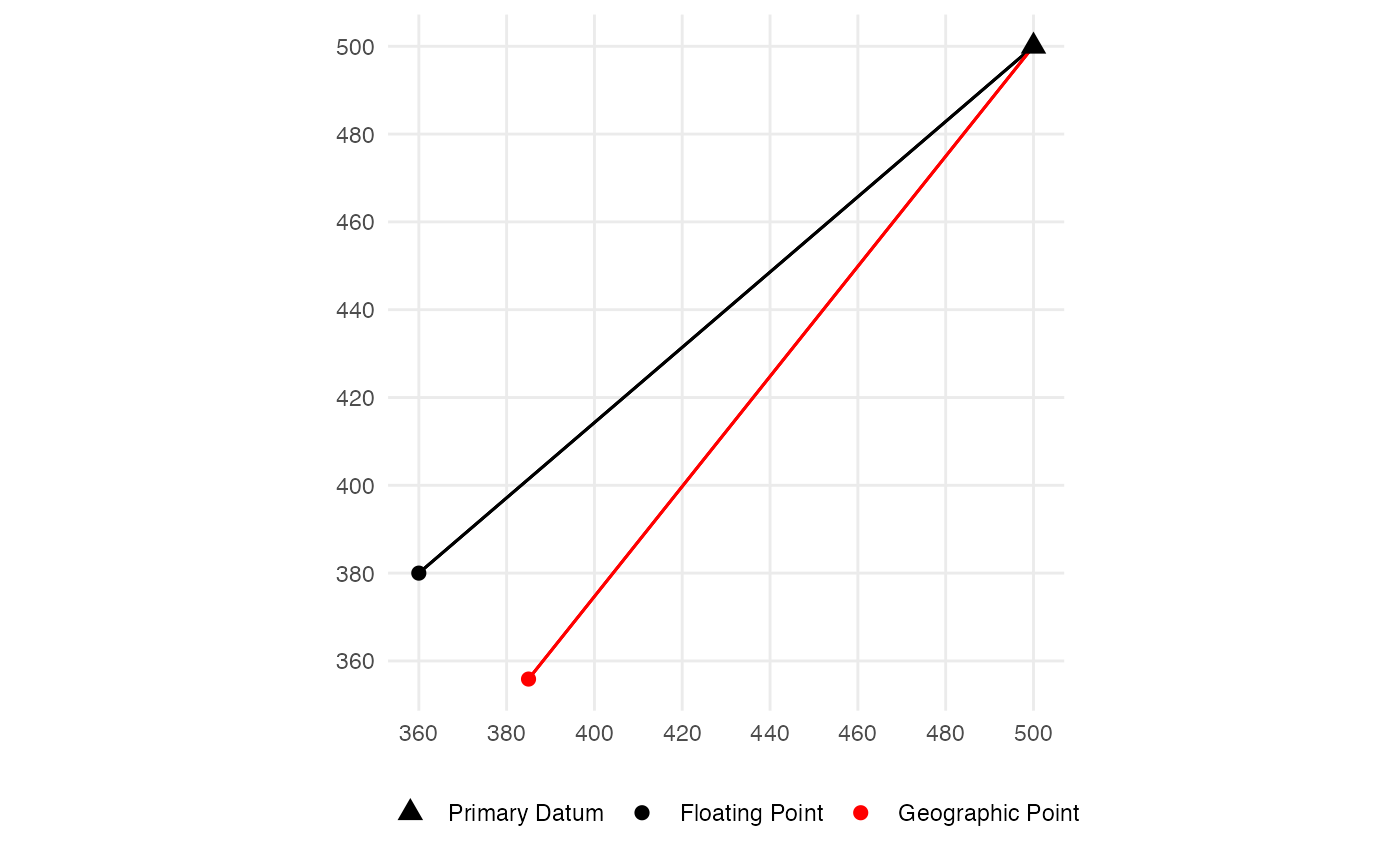
Defining the rotated/scaled OMerc projection
final_omerc <-
  list(proj = "omerc",
       lat_0 = sf::st_coordinates(pts_geo[[1]])[,'Y'],
       lonc = sf::st_coordinates(pts_geo[[1]])[,'X'],
       alpha = alpha_deg,
       gamma = 0,
       k_0 = k_0,
       x_0 = 500,
       y_0 = 500
  ) %>%
  as_proj() %>%
  sf::st_crs()

final_omerc_rounded <-
  list(proj = "omerc",
       lat_0 = sf::st_coordinates(pts_geo[[1]])[,'Y'],
       lonc = sf::st_coordinates(pts_geo[[1]])[,'X'],
       alpha = round(alpha_deg,3),
       gamma = 0,
       k_0 = round(k_0,3),
       x_0 = 500,
       y_0 = 500
  ) %>%
  as_proj()
We can once again define the rotated and scaled OMerc projection using its PROJ definition as +proj=omerc +lat_0=37.385 +lonc=-108.51 +alpha=-10.81 +gamma=0 +k_0=1.299 +x_0=500 +y_0=500. Increasingly, CRSs are being defined using well-known text (WKT) representations of coordinate reference systems. Using R or QGIS, we can view the WKT for our new CRS:
PROJCRS["unknown",
    BASEGEOGCRS["unknown",
        DATUM["World Geodetic System 1984",
            ELLIPSOID["WGS 84",6378137,298.257223563,
                LENGTHUNIT["metre",1]],
            ID["EPSG",6326]],
        PRIMEM["Greenwich",0,
            ANGLEUNIT["degree",0.0174532925199433],
            ID["EPSG",8901]]],
    CONVERSION["unknown",
        METHOD["Hotine Oblique Mercator (variant B)",
            ID["EPSG",9815]],
        PARAMETER["Latitude of projection centre",37.385,
            ANGLEUNIT["degree",0.0174532925199433],
            ID["EPSG",8811]],
        PARAMETER["Longitude of projection centre",-108.51,
            ANGLEUNIT["degree",0.0174532925199433],
            ID["EPSG",8812]],
        PARAMETER["Azimuth of initial line",-10.8099400561365,
            ANGLEUNIT["degree",0.0174532925199433],
            ID["EPSG",8813]],
        PARAMETER["Angle from Rectified to Skew Grid",0,
            ANGLEUNIT["degree",0.0174532925199433],
            ID["EPSG",8814]],
        PARAMETER["Scale factor on initial line",1.29863131831123,
            SCALEUNIT["unity",1],
            ID["EPSG",8815]],
        PARAMETER["Easting at projection centre",500,
            LENGTHUNIT["metre",1],
            ID["EPSG",8816]],
        PARAMETER["Northing at projection centre",500,
            LENGTHUNIT["metre",1],
            ID["EPSG",8817]]],
    CS[Cartesian,2],
        AXIS["(E)",east,
            ORDER[1],
            LENGTHUNIT["metre",1,
                ID["EPSG",9001]]],
        AXIS["(N)",north,
            ORDER[2],
            LENGTHUNIT["metre",1,
                ID["EPSG",9001]]]]